Simplifying Pivot Tables with Timelines and Slicers

How to use Slicers and Timelines to Enhance Data Visualization in Excel

Pivot tables are powerful tools in Microsoft Excel that allow you to analyze and summarize data with ease. In this tutorial, we'll explore how to take your pivot table skills to the next level by adding slicers and timelines to enhance your data analysis. These features make it easier to filter and visualize your data, giving you more control and insights into your Excel spreadsheets. Check out this video to see how to use Timelines and Slicers in your Pivot Tables.

How to insert slicers and timelines into your pivot tables in Excel.

Step 1: Setting the Stage

Before we dive into the details, make sure you have your Excel spreadsheet ready. If you don't already have a pivot table set up, create one by selecting your data and going to the "Insert" tab, then choosing "PivotTable." Once you have your pivot table, you're ready to begin. Refer to this tutorial if you need help creating your Pivot Table.

Step 2: Adding Slicers

Slicers are a fantastic tool to filter data within your pivot table quickly. Here's how to add them:

1. Click on your pivot table.

2. Go to the "PivotTable Analyze" tab in the Excel ribbon.

3. Under "Filters," select "Insert Slicer."

4. A dialog box will appear, allowing you to choose the fields you want to use as slicers. Pick the relevant field, e.g., "Salesperson," and click "OK."

How to Insert a Slicer for your Pivot Table in Excel

Now, you'll see slicer controls for your chosen field, making it easy to filter data dynamically.

Excel Pivot Table Slicer

Step 3: Filtering with Slicers

Once your slicers are in place, you can filter your data:

1. Click on the slicer for the field you want to filter by.

2. Choose one or more items in the slicer by clicking on them or holding down the Ctrl key for multiple selections.

3. Your pivot table will instantly update to reflect your selections, providing real-time insights into the filtered data.

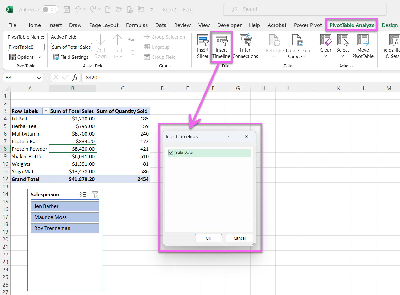
Step 4: Using Timelines

Timelines are excellent for analyzing data over time. Follow these steps to insert a timeline:

1. Click on your pivot table.

2. Navigate to the "PivotTable Analyze" tab in the Excel ribbon.

3. Under "Filters," select "Insert Timeline."

4. Choose the date field you want to use as a timeline and click "OK."

How to Insert a Timeline in your Pivot Table in Excel

You'll now have a timeline control to select specific date ranges.

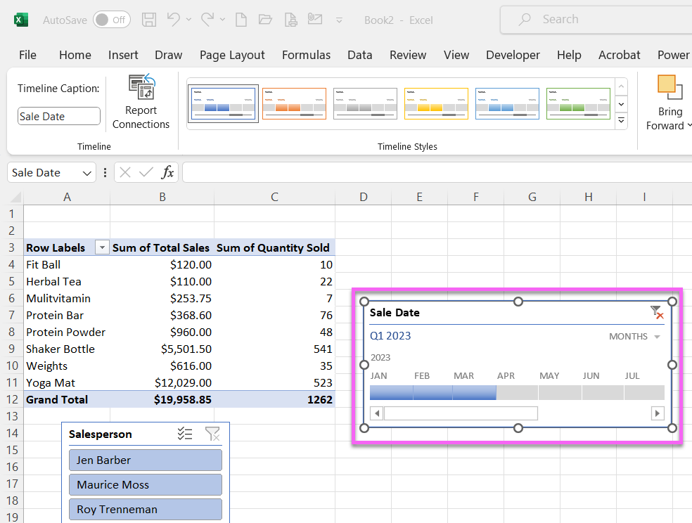
Excel Pivot Table Timeline

Step 5: Analyzing with Timelines

Utilize your timeline to focus on specific date periods:

1. Click on the timeline.

2. Select the date range you want to examine.

3. Your pivot table will automatically update to display data within the chosen time frame.

Conclusion

In this tutorial, we've learned how to supercharge our pivot table skills with slicers and timelines in Excel. These features allow you to filter and visualize data effortlessly, making your data analysis more efficient and insightful. With these tools at your disposal, you'll be able to unlock the full potential of your Excel spreadsheets.

Don't forget to watch the accompanying video for a visual walkthrough of these steps. If you found this tutorial helpful, be sure to explore our other Excel tutorials and subscribe for more valuable tips and insights.