How to Add a Calculated Field to a Pivot Table in Excel

Profit Margin Formula Example

Excel Pivot Tables are powerful tools for data analysis, but what if you need to include a field that doesn't exist in your original dataset? That's where calculated fields come in. In this tutorial, I’ll walk you through the process of adding a calculated field to your Pivot Table in Excel, using a real-world example of calculating Profit Margin. To see this in action you can watch the video here.

How to Add a Calculated Field to a Pivot Table in Excel - Profit Margin Formula Example

Step 1: Prepare Your Data

Before we dive into Pivot Tables, ensure your data is well-organized. A clear header row with descriptive column titles is essential.

Step 2: Create Your Pivot Table

Select Your Data: Click anywhere within your data range.

Insert Pivot Table: Go to the 'Insert' tab and select 'Pivot Table.'

Choose Location: Decide where you want your Pivot Table, and click 'OK.'

How to Insert a Pivot Table in Excel

Step 3: Customize Your Pivot Table

Add Fields: Include the fields you want to analyze. In our case, we'll add 'Product' and 'Total Sales.'

Format Data: Right-click 'Total Sales,' choose 'Currency' for formatting, and click 'OK.'

Step 4: Insert the Calculated Field

Access the Calculated Field Menu: In the Pivot Table Analyze tab, select 'Fields, Items, & Sets,' and click 'Calculated Field.'

Add a Calculated Field to a Pivot Table

Name Your Field: Give your calculated field a name, like 'Profit Margin.'

Build Your Formula: In the formula area, type the formula to calculate Profit Margin: (Total Sales - Cost of Goods Sold) / Total Sales.

Click 'Add' and 'OK': Click 'Add' to create the calculated field and 'OK' to exit.

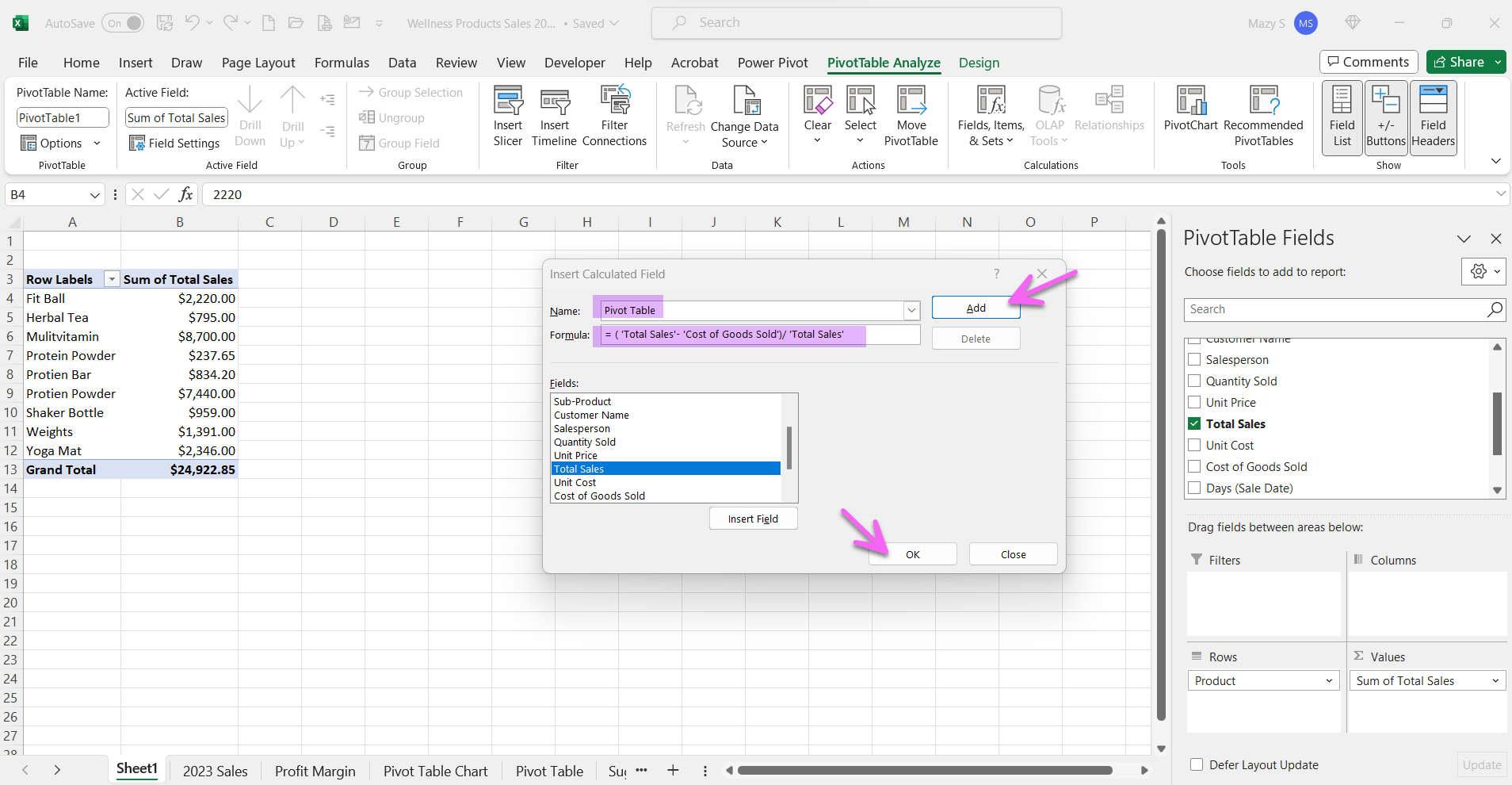
Profit Margin Formula for Calcluated Field in a Pivot Table

Step 5: View Your Calculated Field

Now, you'll see your newly created 'Profit Margin' field in the Pivot Table. It automatically calculates the profit margin for each product.

Step 6: Format as Percentage

Right-Click the Field: Right-click 'Profit Margin.'

Number Format: Choose 'Percentage' to display profit margin as a percentage.

Insert Profit Margin as a Calculated Field in your Pivot Table

Conclusion

Congratulations! You've successfully added a calculated field to your Excel Pivot Table. This technique allows you to extend your data analysis capabilities by including custom calculations that aren't part of your original dataset.

With this newfound knowledge, you can explore various data analysis scenarios and customize your Pivot Tables to suit your specific needs. Excel Pivot Tables become even more versatile when you master calculated fields. Happy data crunching!

Remember, practice makes perfect, so don't hesitate to apply this knowledge to your own Excel projects. Excel's capabilities are vast, and learning how to create calculated fields is just one step toward mastering this powerful tool. Enjoy your data analysis journey!

For more Pivot Table lessons, check out this blog tutorial on Pivot Table Basics and watch the video on Pivot Tables Made Easy to see it in action.